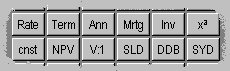
Finance Functions
The financial functions are a powerful tool in making business or personal
financial decisions. To use the financial functions, select Finance from the
Mode menu, or use the keyboard shortcut Ctrl-F, or use shift then the Fin button.. The financial functions allow you to perform all kinds
of financial calculations including the value of investments, the cost of
financing a loan, the discounted value of a future payment or cash flow, and the
equivalent rate of return of a series of payments. There are also buttons to
allow you to quickly add tax, compute a discount or add a mark-up. The meaning
of some of the functions, and the input values needed, are easily forgotten. If
you allow the cursor to hover over a button, or in the case of pen devices if
you do a "tap and hold" with the stylus, a tool tip will appear which gives the
full name of the function and a hint at the order of arguments.
In finance mode the number of decimal places is automatically set to two,
irrespective of the settings in the Option/Display dialog. The display settings
can be modified to change the decimal separator and digit group (thousands)
separator if required. You can select "," or "." for the digit group character
or set it to "no" to disable digit grouping. The scientific and engineering
decimal display settings also have no effect.
The example below assume that you are using Algebraic logic. For RPN logic
you will need to alter the keystrokes slightly. So for example if the key
sequence given is 100 func 200 = , for RPN
you would use 100 Ent 200
func.
Whilst we have taken every care to ensure that these calculator functions and
the descriptions are accurate, we must remind you that you use them at your own
risk. If you are in any doubt, you are urged to seek professional financial
advice before making major financial decisions.
Using the percent key
The percent key is available in most modes and works in exactly the same way.
In this section we show how you might use it for financial calculations. To get
the percent key use the shift and = buttons. This displays the result of an arithmetic operation as a percentage.
Examples:
Calculate the tax at 17.5% on � 25.00:
250 x 17.5 shift %
Result: �
43.75
Calculate 12% mark-up on $250
250 + 12 shift %
Result: $ 280
Give 5% discount on goods costing $125
125 - 5 shift %
Result: $ 118.75
Using the tax, before tax b/t, discount d/c and mark-up m/u functions.
The percentage calculations described above can be performed more
conveniently using the special keys available in finance mode. The tax, discount
(d/c) and mark-up (m/u) functions all do this automatically, without needing a
percentage to be entered. The percentage rates you regularly use will typically
not change frequently and these can be programmed in to the calculator. Any time
you need to use an ad-hoc percentage in a calculation you can revert to using
the percentage key.
First, here is how to change the percentages. Click on the rate button to bring up the financial rates dialog box. We will look at this
dialog further in the following sections. It shows you the rates used by various
functions. To change the tax, discount or mark-up rates, select the appropriate
edit box and enter the new percentage (on Pocket PC devices the input window
should come up automatically). So, supposing that the sales tax (or value added
tax) rate is 17.5%, we would enter this value for the tax rate. Similarly, if we
regularly offer customers a 20% discount, we would enter that value as the
discount percentage. (Do not confuse the discount percentage with the discount rate, a separate percentage rate which is used in depreciation
calculations). If we use regularly use a mark-up of 40% on goods, we would enter
this value also. Click on the OK button when you are finished with the rates
dialog.
Once the rates have been set you can use the Tax, d/c and m/u buttons to
quickly perform percentage calculations. The tax and mark-up buttons compute the
result of adding the tax or mark-up percentage. The discount button computes the
amount after subtracting the discount percentage. The before tax (b/t) button
can be used to calculate the tax-exclusive amount from a given tax-inclusive
total.
Example: calculate the 17.5% VAT inclusive price of an item costing �
99 excluding VAT.
First set the tax rate to 17.5%.
Enter the amount - 99.0
Click on the tax button: result: 116.32
Example: calculate the VAT exclusive price of an item with a retail
VAT inclusive price of � 99.
If needed, check that the tax rate is set to 17.5%.
Enter the amount - 99.0
Click on the shift button then the b/t (before tax)
button: result: �
84.26
Setting Interest and Discount Rates Rate
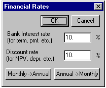
To choose the various percentage rates used in financial calculations, use
the Rate button which brings up the Financial Rates dialog box. The
dialog box can also be used to convert between nominal and effective rates for
different interest payment schedules.
The bank interest rate is applied to the loan calculations (Loan, Savg, TM, TMa, PV, PVa, FV and FVa) and the discount rate to the Net Present Value calculations (NPV and VFl ). Typically these will be assigned different values which prevail at the time
of the calculation and to the relevant field of commerce. The rates also vary
between financial institutions, and depending on whether you are dealing with a
loan or savings, and between different financial products from the same
institution.
By default it is assumed that the period in these calculations is annual. In
this case there is no difference between the nominal interest rate and the
effective interest rate. If a different period is required then the Period:
drop-down list box can be used to select biannual, quarterly, monthly, weekly or
daily interest payments. The nominal or effective annual rate can be used to
specify the interest rate by entering a value in the input box - if the nominal
rate is entered the effective rate is automatically calculated and displayed in
the adjacent edit box and vice versa. The effective rate is the annual rate of
interest taking into account the compounding of the individual payments over the
year, and is sometimes referred to as the Annual Effective Rate (AER) or Annual
Percentage Rate (APR - this sometimes is used to include additional related
finance charges). Because of compounding this rate will be slightly higher than
the nominal annual rate. Banks may quote both rates, and lenders are often
legally obliged to display an APR as well as the lower nominal rate which they
tend to give prominence.
Changing the period automatically updates the effective rate. If you change
the nominal rate the effective rate is updated automatically, so you can use
this to work out the effective rate for a given nominal rate and period. You can
also work back to the nominal rate for a given effective rate by changing the
value in the effective rate box, which automatically updates the nominal rate.
This can be useful if a lender or savings institution quotes one of these rates
but not the other.
If the payment is made at the end of each period, the arrears radio
button should be selected. If the payment is made at the beginning of each
period, select the advance radio button. Don't forget that the financial
functions expect a number of periods, so for example if the period is monthly
then five years is 5 x 12 = 60 periods.
The Financial Rates dialog box also allows you to specify the tax, markup and
discount rates used by the Tax and m/u and d/c functions.
Example: A lender quotes an annual rate of 6% for a loan, but interest
is payable monthly. What is the effective annual rate?
The lender will charge interest at 6% divided by 12 months, or 0.5% per
month. The total interest paid per year will be 6% of the capital, but because
of the time value of money it is more expensive than paying this amount at the
end of the period. To get the effective interest rate, open the Rates dialog and
enter 6 for the nominal bank rate and select "monthly" from the period drop-down
box. The effective rate is automatically updated to show 6.16778%. If the lender
had quoted "6% APR" you could work back to the nominal rate by entering this in
the effective rate box, and the nominal rate would show 5.84106%.
Time Value of Money Calculations
The following group of functions are concerned with the time value of money,
and the present or future value of a fixed amount or a series of regular
payments. This includes loan calculations, mortgages and annuities. The three
functions TM, PV and FV are used to calculate the term, present and future
values of fixed amounts. They each have a corresponding annuity function which
is used to compute the term, present or future values of a series of regular
payments. The word "annuity" is used in this context in a general sense meaning
any recurring regular payment. The payment is not necessarily an annual one, and
not necessarily a regular income purchased for a fixed price as in pensions
planning.
These functions all use the bank rate to compute time-dependent values. The
period defaults to one year but can also be set to be biannual, quarterly,
monthly, weekly or daily. The bank rate and period are set in the Rate dialog box. This dialog can also be used to define whether payments are made or
received at the beginning or end of each period.
Savg Savings Payment
To compute the periodic payment needed to accumulate a given amount, enter
the final amount (future value), click the Savg button, then enter the term
(number of payments). Press =
to get the amount of each payment.
Example: You decide to start saving for a holiday in 12 months time.
How much should you save each month in order to have �1000 available at the end
(assuming 10% bank rate)? What total amount must you put aside?
Check that the bank rate is set at 10% and that the period is monthly,
payment in advance.
1000 Savg 12 = Result: 78.92
X 12 = Result: 947.10
The total amount saved is � 947.10. The interest earned makes the amount up
to � 1000.
Loan Loan Payment
To compute the required periodic payments to repay a given loan, enter the
amount of the loan (present value), click the Loan
button, then enter the term (number of payments). Press =
to get the amount of each payment.
Usually the term of a mortgage is defined in years, but the repayment periods
and corresponding calculations are carried out monthly.
Example: What is the monthly payment to pay off a loan of $30,000
dollars over 25 years at an interest rate of 10% ?
First click on Rate to check that the interest rate is set to 10% (and change it if needed),
and set the period of the payments to monthly. You can note that the effective
interest rate changes to about 10.47%. You should also set the payments to
"arrears", assuming you will be paying the mortgage at the end of each month.
The period is now in months, which over 25 years is 25x12 months (i.e. 300
months).
3 0 0 0 0 Loan ( 2 5 X 12 ) =
Result: $ 272.61 (the monthly payment).
Int Calculate Interest Payments
To calculate the interest payment, per period, on a loan or saving, enter the
loan or investment amount, then shift and then Int .
Example: Your business borrows $500,000. What is the monthly interest
payment?
Check your rates (e.g. use 10%, monthly payment).
500000 Int Result: 4166.67 - the monthly interest payment.
TM Term of Investment
To compute the term required for an investment to increase to a given value,
enter the principal, followed by TM followed by the desired compounded sum at the term. The result is the number
of periods (generally years) required for the investment to reach this value. If
you wish to use a different period (monthly for example) you need to change the
value of the interest rate accordingly, by pressing Rate .
Example: How many years of annual compound interest are required for
an initial investment of $100 to reach the value of $200 (assuming 10% bank
interest rate)?
First make sure the bank rate is set to 10% and the period is set to annual
1 0 0 TM 2 0 0 =
Result: 7.27 (i.e. 8 years to exceed $200).
TMa Term of an Annuity
To compute the term required for a series of regular payments to increase to
a given value, enter the payment, followed by TMa followed by the
desired compounded sum at the term.
Example: You plan to buy a boat costing $20000. You can afford to save
$300 per month. How long will it take to save for the boat (assuming 7% bank
interest over the period, and monthly compounding, payment in advance)?
First check the rate and period are set correctly in the Rate dialog.
300 TMa 20000 =
Result: 56.20
The number of periods is 56.2, or about 4 years and 9 months.
PV Present Value of an Investment
This function computes the present value of a future amount. This can be used
to find out how much you would need to invest now to be worth some specified
amount in the future. You can also use it to work out the present value of some
future amount. This can be useful if you need to compare alternative investments
which yield amounts at different times in the future.
Example: Which is worth more now; � 500 in two years time, or � 1000
in ten years time?
To answer this we need to make a guess of the interest rate over the next ten
years or so. Let's assume this to be 5% and, for argument's sake, compounded
annually. We can then work out the present value of the two future amounts so
that we can make a comparison.
500 PV 2 = Result: 453.51
1000 PV 10 = Result: 613.91
This suggests that the � 1000 is worth waiting for. In practice you might
take into account any commercial risk of default on the payment over the longer
period.
Example: You plan to give a four year old child $1000 on their
eighteenth birthday. What amount do you need to invest today (assuming 7% bank
interest over the period, and monthly compounding)?
First check the rate and period are set correctly in the Rate dialog.
1000 PV ( 14 X 12 ) =
Result: 376.38
One problem with such long term calculations is that the bank rate will very
probably vary a great deal over a long period. In this case it is necessary to
use a guess of the likely average rate over time based on historical interest
rates. It would also be wise to choose a fairly conservative value for the
expected interest rate.
PVa Value of Annuity
To calculate the present value of an annuity at maturity, enter the amount of
the payment, then FVa , followed by the term (number of periods). Despite the literal meaning of the
word annuity, it is possible to use a period other than annual in the
calculation, in which case you need to change the value of the interest rate
accordingly, by pressing Rate .
Example: You decide to finance the purchase of a car costing $15,000
over a period of five years, but can only afford a monthly payment of $300. If
the finance company offers an APR of 10% compounded monthly, what down payment
would be required?
Make sure rate is 10%, period is monthly, payment in arrears.
300 PVa ( 5 X 12 ) =
Result: $ 14119.61
- 15000 =
Result: $ -880.39
A down payment of $880 is required.
FV Future Value of an Investment
To compute the value of a single amount invested for a given number of years
at the current interest rate, enter the principal, click FV and the
number of investment periods. Usually the number of periods is the number of
years. If you wish to use a different period (monthly for example) you need to
change the value of the interest rate accordingly, by pressing Rate .
Example: What is the value of $100 invested for five years at compound
interest (assuming a 10% annual interest rate)?
First check that the Rate dialog is set to the correct bank rate (10%) and
period (annual).
1 0 0 FV 5 =
Result: $161.05
You can also compute the value of the same investment if interest is computed
monthly by setting the period to monthly in the Rate dialog and
adjusting the number of periods accordingly:
1 0 0 FV ( 5 X 12 ) =
Result: $ 164.53
FVa Future Value
of Annuity
To calculate the future value of an annuity at maturity, enter the amount of
the annual payment, then FVa , followed by the term (number of periods).
Despite the literal meaning of the word annuity, it is possible to use a
period other than annual in the calculation, in which case you need to change
the value of the interest rate accordingly, by pressing Rate .
Example: What is the value at maturity of a 30 year annuity with an
annual payment of $200 (assuming an interest rate of 10%)?
Make sure rate is 10%, period is annual, payment in advance.
2 0 0 FVa 3 0 =
Result: $ 36188.68
Cash Flow Functions
Cash flow functions are designed to compute the present value of an irregular
series of payments. These functions use the discount rate in the Rate dialog box. In order to use the IRR and VFl functions you will need to set the
calculator to array mode. To do this, select the Option/Matrix menu and set the
grid to the desired size, and check the box labelled "Show matrix in all modes".
If the array is two-dimensional, the values corresponding to successive periods
are ordered right to left in rows, and then row by row from top to bottom.
IRR Internal Rate of Return
The internal rate of return is the discount rate at which the present value
of a series of payments would be zero. The practice is to compare this with the
bank rate to decide whether the investment is preferable to simply investing the
capital in a bank. In real situations there is usually an element of risk and
uncertainty in the expected future payments and this should be taken into
account when making investment decisions.
To compute the internal rate of return on an irregular series of payments,
first select the Option/Matrix menu and set the grid to the desired size, and
check the box labelled "Show matrix in all modes". Then enter the values of the
payments into the array (if the array is two-dimensional, remember that the
elements are ordered from left to right and then from top to bottom). The
investments should be entered as negative numbers. Make sure all cells are
selected and then click on the IRR button to get the IRR value.
It is possible for a set of cash flows to exist for which there is no IRR, or
for the value to be too large or negative, in which case an overflow error is
displayed.
Example: You plan to invest $1000 and expect to receive nothing in the
first year, $100 in the second year, $200 in the third year, and then $300 in
the fourth, fifth and sixth years. What is the internal rate of return?
Enter the values -1000, 100, 200, 300, 300, 300 into the array (make sure all
cells are selected when you finish). Then click on the IRR button.
The array is filled with the internal rate of return, which is computed as
5.55 .
NPV Calculate Net Present Value of a Future Cash Flow
To calculate the present value of an amount to be paid at some time in the
future, enter the value of the amount, followed by NPV and then the number of periods before the payment will be made. The length of
the period is determined by the settings in the Rate dialog box, and
defaults to one year. If you wish to use a different period (monthly for
example) you need to change the value of the period accordingly.
The NPV function is exactly the same as the PV function
except that it uses the discount rate instead of the bank rate.
You can enter a negative number of periods, in which case you get the present
value of a payment which was paid at some time in the past. If you require the
net present value of a series of periodic cash flows, use PVa taking
care to set the bank rate to the required discount rate. Alternatively use the VFl function with equal amounts.
Example: What is the net present value of $100 to be paid in five
years time (assuming 5% discount rate).
First check that the discount rate is set to 5%; period to annual.
1 0 0 NPV 5 =
Result: $ 78.35
VFl Net Present Value of Cash Flows
To calculate the net present value of a series
of uneven cash flows, first select the Option/Matrix menu and set the grid to
the desired size, and check the box labelled "Show matrix in all modes". Next
enter the cash flow for each period into the array. Make sure that all cells are
selected and press the VFl button. The array is now filled with the
net present value for each corresponding period. The value corresponding to the
last entry is the present value of the whole cash flow.
Typically the period is annual. If you wish to use a different period
(monthly for example) you need to change the value of the discount rate
accordingly, by pressing Rate .
Example: A project requires an initial capital expenditure of
$1,000,000. After five years the capital equipment is to be written off. The
expected annual revenue stream at the end of each year, less running costs, is:
year 1 - $100,000; year 2 - $200,000, year 3 - $300,000, year 4 - $300,000, year
5 - $300,000. The net revenues exceed the initial capital cost, but is the
investment a good one, assuming a discounting rate of 5% per annum?
Input the values, with a value of zero for year 1:
0.00
100000.00
200000.00
300000.00
300000.00
300000.00
VFl
Result:
0.00
95238.10
276643.99
535795.27
782606.01
1017663.86
The result shows that, taking into account the time value of money, the
revenue flows have a net present value of $1017663.86, so that the project is
just profitable (but probably not worth the risk!).
Depreciation Functions
The depreciation functions compute a depreciation factor for a given asset
life (in periods) and number of periods. For example, the depreciation factor
for an asset with a life of 10 years after 5 years with straight line
depreciation would be computed as 1 0 SLD 5. The resulting factor, 0.5, can be applied to the
value of the asset less any salvage value at the end of the period.
SLD Straight Line Depreciation
To calculate the fraction of the value of an asset which is depreciated after a
given time using straight-line depreciation, enter the initial cost less any
salvage value, then X , followed by the useful asset life, then SLD , followed by the number of periods after which the depreciation is to be
calculated, followed by = . The result is the total
(cumulative) depreciation charge.
Usually the number of periods is the number of years. If you wish to use a
different period (monthly for example) you need to change the value of the
discount rate accordingly, by pressing Rate .
Example: What is the depreciation after five years on a capital asset
costing $10,000 with a ten year life and a salvage value of $1000 at the end of
its life?
1 0 SLD 5 =
Result: 0.50 (the depreciation factor)
X
(
1 0 0 0 0 -
1 0 0 0 )
=
Result: 4500.00
The depreciation is $4500, therefore the value of the asset after 5 years is
$10000 - $4500 = $5500.00
Using RPN logic, you would enter:
10000 Ent 1000 - 10 Ent 5 SLD X
DDB Double declining Balance
Depreciation
The double-declining balance method of depreciation is an accelerated
depreciation method which provides more rapid depreciation charges in the early
part of the lifetime of the asset. This method is often preferred when
calculating depreciation charges for tax purposes, for example. To calculate the
fraction of the value of an asset which is depreciated after a given time using
the double-declining balance method of depreciation, enter the initial cost
(ignoring the residual value), then X , followed by the useful asset life, then DDB , followed by the number of periods after which the depreciation is to be
calculated, followed by = . The result is the total (cumulative)
depreciation charge.
Usually the number of periods is the number of years. If you wish to use a
different period (monthly for example) you need to change the value of the
discount rate accordingly, by pressing Rate .
Example: What is the depreciation after five years on a capital asset
costing $10,000 with a ten year life and a salvage value of $1000 at the end of
its life?
(
1 0 DDB
5 )
X
1 0 0 0 0 =
Result: 6723.20
The depreciation is $6723, therefore the value of the asset after 5 years is
$10000 - $6723 = $3277
Applying the depreciation to the whole of the asset value, rather than the value
less the residual value, results in a faster rate of depreciation (which is
usually advantageous). This does mean that the depreciation charge may bring the
depreciated value below the residual value near the end of the life of the
asset. When this happens the usual practice is to reduce the depreciation charge
to a value which leaves the residual value and allow the asset to remain at this
value until it is sold or disposed of.
SYD Sum-of-Years-Digits Depreciation
The Sum-of-Years-Digits is another accelerated depreciation method. To
calculate the fraction of the value of an asset which is depreciated after a
given time using sum-of-years-digits, enter the initial cost less any salvage
value, then X
, followed by the useful asset life, then SYD
, followed by the number of periods after which the depreciation is to be
calculated, followed by = . The result is the total (cumulative)
depreciation charge.
Usually the number of periods is the number of years. If you wish to use a
different period (monthly for example) you need to change the value of the
discount rate accordingly, by pressing Rate .
Example: What is the depreciation after five years on a capital asset
costing $10,000 with a ten year life and a salvage value of $1000 at the end of
its life?
1 0 SYD 5 =
X ( 1 0 0 0 0 - 1 0 0 0 ) =
Result: 6545.45
The depreciation is $6545, therefore the value of the asset after 5 years is
$10000 - $6545 = $3455
Currency Conversion
You can use the conversion feature to perform conversions between some of the
major currencies and the former currencies of the European Union. Select
"Currency" as the property and then select the To and From currencies from the
drop-down lists. Apart from the former currencies of countries now using the
Euro (which had a fixed exchange rate) the currency conversions fluctuate and so
the conversions will not be up-to-date. The date at which the conversion was set
is indicated for each currency. You can get updated currency files from time to
time at our web site (http://www.calculator.org/),
or you can edit the currency conversions yourself as needed.
For more information on using the conversion utility see the
relevant section.
More examples
Example: You have $100,000 in a savings account, earning 6% annual interest, credited
monthly. In addition, $500 is deposited every month. How long will the funds
last if $1,500 is withdrawn every month?
That's a net withdrawal of $1000/month (the withdrawal and deposit amounts can
be offset). Interest is 0.5%/month (or you could correct for compounding if
appropriate). None of the built-in functions yield a term for an annuity type
investment, but we can use the formula:
Term = - log(1 - PV.rate/pmt) / log(1 + rate)
where PV (present value) is 100000 and pmt (payment) is 1000 so
Term = - log(1 - 100000 x 0.005 / 1000) / log(1 + 0.005)
= 138.975 months, or about 11 1/2 years.
You can check this value using the Mortgage function by computing the mortgage
repayment on a $100000 loan over 139 months, which gives a payment of about
$1000. You can also check using the Annuity function that a $1000 payment over
139 months yields about $200000, if the rate is set to 0.005%. You can then
discount this to the present value (using NPV with a term of 139) to get back to
about $100000.
Example: In the above example, how much can be withdrawn each month to
make equal monthly withdrawals for 10 years?
This can be done using the Mortgage function, entering the principal amount and
the term (i.e. $100000 and 120 months). The result should be $1110.21 per month.
If you are paying in $500 per month also, you can simply offset that with the
withdrawal.
Example: You have a $50,000 mortgage payable over 30 years. How does the
balance change over this period.
First select the Option/Matrix menu and set the grid to 12 x 30, and check the
box labelled "Show matrix in all modes". Switch to Matrix mode and click on the
shift and ind buttons to fill the array with indices then
- 359 = +/-
to reverse the order. Use
Min to save the values for later use. Switch back to Finance mode.
Set the rate to 5%, the period to monthly, and select "Arrears". Calculate the
monthly payment:
50000 Loan ( 30 X
12 ) = Result:
268.41 (in all cells)
 </p>

 <p>
Now calculate the present values:
shift PVa MR =
The result will be the balance outstanding after each period, with
    months along the x-axis and year number on the y-axis. The balance falls

    slowly at first and decreases rapidly near the end to zero when the

    mortgage is paid off.</p>

 <p>
Comparison of the Various Financial Functions
For time value of money calculations, the variables are the interest rate,
the period, whether the payment is at the beginning or end of the period
(advance or arrears), the periodic payment (PMT), the present value (PV), the
future value (FV) and the term. Normally the interest rate and period are fixed
(in the case of this software by the Rates dialog). Therefore if three of PMT,
PV, FV and TERM are known the other can be calculated. In addition in most
calculations one of the four is zero leaving two unknowns.
The table below shows the various functions available with the unknown
quantities indicated by an "x", a zero showing the fixed zero value, and "ans"
to indicate the value computed by the function.
| Legend | Function | PMT | PV | FV | TERM | Rate |
|---|---|---|---|---|---|---|
| TM | Term of Inv. | 0 | x | x | ans | B |
| TMa | Term of Ann. | x | 0 | x | ans | B |
| PV | Present Value | 0 | ans | x | x | B |
| PVa | Present Value of Ann. | x | ans | x | B | |
| FV | Future Value | 0 | x | ans | x | B |
| FVa | Future Value of Ann. | x | 0 | ans | x | B |
| Loan | Loan Payment | ans | x | 0 | x | B |
| Savg | Savings Payment | ans | 0 | x | x | B |
| NPV | Net Present Value | 0 | ans | x | x | D |
| Int | Interest | 0 | x | n/a | n/a | B |
If you need to compute any of the various quantities by hand, the
underlying arithmetic functions are as follows (r = rate):</p>
<p>TM(PV, FV) = log(FV/PV)/log(1+r)</p>
<p>TMa(PMT, FV) = log(1 + FV.r/PMT) / log(1 + r)</p>
<p>PV(FV, term) = FV.(1 + r)<sup> -term</sup></p>
<p>PVa(PMT, term) = PMT.(1 - (1+r)<sup>-n</sup>) / r or PMT.(1 + r).(1 - (1
+ r)<sup>-n</sup>) / r (advance)</p>
<p>FV(PV, term) = PV.(1 + r)<sup> term</sup></p>
<p>FVa(PMT, term) = PMT.((1 + r)<sup> term</sup> - 1) / r or PMT.(1 +
r).((1 + r)<sup> term</sup> - 1) / r (advance)</p>
<p>Loan(PV, term) = PV.r / (1 - (1 + r) <sup>-term</sup>) or PV.r / (1 - (1
+ r) <sup>-term</sup>) / (1 + r) (advance)</p>
<p>Savg(FV, term) = FV.r / ((1 + r) <sup>term</sup> - 1) or FV.r / ((1 + r) <sup>
term</sup> - 1) / (1 + r) (advance)</p>
<p>NPV(FV, term) = FV.(1 + r<sub>d </sub>)<sup>
-term</sup></p>
<p>V<sub>flow</sub> (FV<sub>n</sub>) = <font face="Arial"><font size="5">Σ</font>
FV<sub>n</sub>.(1 + r<sub>d</sub>)
<sup>-n</sup></font></p>
<p><font face="Arial">Int(PV) = PV.r</font></p>
<p>